A regression analysis is a statistical analysis method that examines the relationships between two variables.
These are a dependent variable Y (also called the outcome variable) and an independent variable X (also called the influencing variable). Regression analyses are always used when correlations need to be described or predicted in terms of quantities. Mathematically, the influence of X on Y is symbolized by an arrow:
X → Y
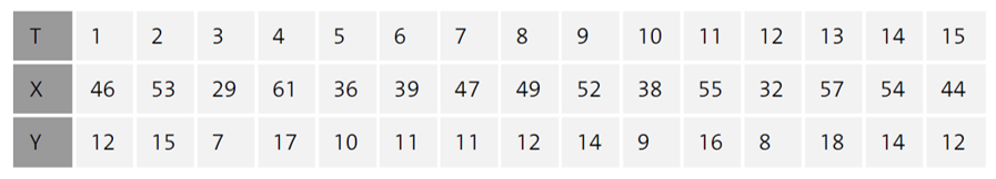
I want to use a simple example to describe the regression analysis method: In a storage room for synthetic fibers, there is a certain relative humidity. Over a period of 15 days, the relative humidity of the room (X) and the moisture content of the synthetic fiber (Y) are measured once a day. A regression analysis will be used to investigate whether there is a correlation between these two variables and, if so, how strong this correlation is. In this table, the measurement values are documented.
In the simplest case, a linear relationship exists between the X and Y values, which can be described by a linear function with the slope m and the intercept a of the function line with the y axis:
y = mx +a
The m and a parameters are also referred to as regression parameters. The strength of the correlation between X and Y of the two measurement series is determined by the correlation coefficient r.
Computing the Regression Parameters
The correlation coefficient r is defined as the quotient of the covariance sxy of two measurement series and the product of the standard deviations, sxsy:

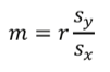
The slope of the regression line is the quotient of the covariance and the square of the standard deviation of the x-values:
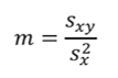
The slope can also be calculated using the correlation coefficient:
The intercept of the regression line is computed from the difference of the mean value of all y-values and the product of the slope m with the mean value of all x-values:
![]()
All regression parameters can be computed directly using the following SciPy function:
m,a,r,p,e = stats.linregress(X,Y)
The return values p and e of the tuple are not needed for computing the regression parameters.
The listing below calculates the slope m, the y-axis intercept a of the regression line and the correlation coefficient r for the measurement values listed earlier. To show the different options of Python, the parameters are calculated and compared by using the corresponding NumPy and SciPy functions.
01 #14_correlation.py
02 import numpy as np
03 from scipy import stats
04 X=np.array([46,53,29,61,36,39,47,49,52,38,55,32,57,54,44])
05 Y=np.array([12,15,7,17,10,11,11,12,14,9,16,8,18,14,12])
06 xm=np.mean(X)
07 ym=np.mean(Y)
08 sx=np.std(X,ddof=1)
09 sy=np.std(Y,ddof=1)
10 sxy=np.cov(X,Y)
11 r1=sxy/(sx*sy)
12 r2=np.corrcoef(X,Y)
13 m1=sxy[0,1]/sx**2
14 m2=r2[0,1]*sy/sx
15 a1=ym-m2*xm
16 m3, a2, r3, p, e = stats.linregress(X,Y)
17 print("NumPy1 slope:",m1)
18 print("NumPy2 slope:",m2)
19 print("SciPy slope:",m3)
20 print("Intersection with the y-axis:",a1)
21 print("Intersection with the y-axis:",a2)
22 print("Def. correlation coefficient:",r1[0,1])
23 print("NumPy correlation coefficient:",r2[0,1])
24 print("SciPy correlation coefficient:",r3)
25 print("Estimated error:",e)
Output
NumPy1 slope: 0.32320356181404014
NumPy2 slope: 0.3232035618140402
SciPy slope: 0.3232035618140402
Intersection with the y-axis: -2.5104576516877213
Intersection with the y-axis: -2.5104576516877213
Def correlation coefficient: 0.9546538498757964
NumPy correlation coefficient: 0.9546538498757965
SciPy correlation coefficient: 0.9546538498757965
Estimated error: 0.027955268902524828
Analysis
Lines 04 and 05 contain the measurement values for the relative humidity X and the moisture content of the material Y. The program computes the regression parameters from these measurement values and uses the correlation coefficient to check whether a correlation exists between the influencing variable X and the outcome variable Y and to determine how strong this correlation is.
Line 10 computes the covariance sxy using the np.cov(X,Y) NumPy function. This function returns a 2 × 2 matrix. The value for sxy is either in the first row, second column, of the matrix or in the second row, first column, of the matrix. The correlation coefficient r1 is then calculated with sxy in line 11.
A simpler way to calculate the correlation coefficient is to directly use NumPy function np.corrcoef(X,Y) (line 12). This function also returns a 2 × 2 matrix. The value for r2 is either in the first row, second column, of the matrix or in the second row, first column of the matrix.
Line 13 calculates the slope m1 from the covariance sxy[0,1] and the square of the standard deviation sx from the X measurement values. The slope m2 is calculated in line 14 using the correlation coefficient r2(0,1) and the standard deviations sx and sy.
In line 15, the y-axis intercept a1 is calculated from the mean values of the X and Y values using the conventional method. Instead of the slope m2, the slope m1 could have been used as well.
The most effective method to calculate all three parameters with only one statement is shown in line 16. The slope m3, the y-axis intercept a2, and the correlation coefficient r3 are returned as tuples by the SciPy function stats.linregress(X,Y).
The print() function outputs the regression parameters in lines 17 to 25. All computation methods provide the same results. The slope is about 0.32, and the y-axis intercept has a value of about −2.51. Thus, the regression line adheres to the following equation:
![]()
The correlation coefficient of r = 0.95465 is close to 1. Thus, a strong correlation exists between the relative humidity (X) and the moisture content of the material (Y).
Representing the Scatter Plot and the Regression Line
When the discrete yi values of the Y measurement series and the discrete xi values of the X measurement series are plotted in an x-y coordinate system, this plot is referred to as a scatter plot. This listing shows how to implement such a scatter plot with the values listed in our table and the corresponding regression line.
01 #15_regeression_line.py
02 import numpy as np
03 import matplotlib.pyplot as plt
04 from scipy import stats
05 X=np.array([46,53,29,61,36,39,47,49,52,38,55,32,57,54,44])
06 Y=np.array([12,15,7,17,10,11,11,12,14,9,16,8,18,14,12])
07 m, a, r, p, e = stats.linregress(X,Y)
08 fig, ax=plt.subplots()
09 ax.plot(X, Y,'rx')
10 ax.plot(X, m*X+a)
11 ax.set_xlabel("Relative humidity in %")
12 ax.set_ylabel("Moisture content of the material")
13 plt.show()
Output
This figure shows the output regression line after the calculation.
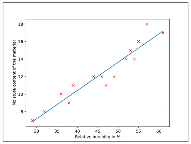
Analysis
The program determines the y-axis intercept a and the slope m in line 07 using the stats.linregress(X,Y) SciPy function. Line 09 plots the discrete xi and yi values as red crosses using the plot(X, Y, 'rx') method. The ax.plot(X, m*X+a) statement in line 10 causes the plot of the regression line. The crosses of the scatter plot clearly show that a strong correlation exists between the relative humidity and the moisture content of the material.
Editor’s note: This post has been adapted from a section of the book Python for Engineering and Scientific Computing by Veit Steinkamp. Dr. Steinkamp studied electrical engineering and German to become a teacher and pass on his knowledge at vocational schools and technical colleges. He teaches electrical engineering, application development, and mechanical engineering technology. He has also taught theoretical electrical engineering and the fundamentals of electrical engineering.
This post was originally published 4/2024.


Comments