

Once you've loaded data from a file into a pandas DataFrame, the next step is to perform data cleaning.
This involves filtering, preparing, and transforming the data so that it can be easily analyzed, visualized, and processed further. While this is sometimes time-consuming because it usually requires many steps, pandas offers practical tools for everything, which we’ll now take a look at.
Filtering Data
I have a pandas DataFrame containing Date, Location, Temperature_F, and Precipitation_ in. I only need the data from Seattle.
You can easily filter the DataFrame for Seattle. Assuming your DataFrame is named df and the column containing the location is named Location, do the following:
df_seattle = df[df["Location"] == "Seattle"]
Filtering is very easy with pandas, as you can use the syntax with a filter predicate in square brackets. This even allows you to combine multiple conditions using & (and) and | (or). It’s important with such complex predicates that they are always enclosed in parentheses:
df = df.loc[(df["Location"] == "Seattle") & ((df["Temperature_F"] < 50)
| (df["Temperature_F"] > 80)) ]
Earlier, we assigned the DataFrame to a new variable df_seattle; in this example, we’ve simply overwritten the original DataFrame df.
Since we now only have climate data from Seattle after filtering, we no longer actually need the Location column. We could now delete it using df.drop(columns="Location"); alternatively, we can also specify which columns we want to keep directly during filtering:
df = df.loc[df["Location"] == "Seattle",
["Date", "Temperature_F", "Precipitation_in"]]
Identifying and Handling Missing Values
When we looked at general information and statistics about the DataFrame earlier using df.info() and df.describe(), we could already see how many records actually had a value in a given column.
For the following examples, let’s simply set the temperature in the first row to “unknown” (None):
df.loc[0, "Temperature_F"] = None
If we examine the DataFrame using df or print(df), we now see the value NaN (not a number) in the first row of the Temperature_F column. Such missing data occurs quite frequently in practice. Therefore, the task now is to identify it and then consider how to handle it.
The isna() method can be applied to a Series (i.e., a single column) or to an entire DataFrame. It returns a Series or a DataFrame where True appears wherever a value was previously missing; the other entries now show False. Using the sum method, we then count the number of True values, that is, the missing values:
print(df.isna().sum()) # Number of missing values per column
print(df["Temperature_F"].isna().sum()) # … or just in this column
One possible solution for handling missing values is to simply delete the entire rows containing gaps:
df = df.dropna()
After that, every row where a value is missing in any column is gone. However, with df.dropna(subset=["Temperature_F"]), you can also specify that only certain columns should be checked.
Instead of deleting the rows, we can also simply fill in the missing values:
df = df.fillna({
"Temperature_F": df["Temperature_F"].mean(),
"Precipitation_in": 0,
"Date": "2026-01-01"
})
Wherever the temperature is missing in our sample dataset, it’s set to the average value of the entire column. If a precipitation value is missing anywhere, we set it to 0. For missing values in the date column, we simply choose January 1, 2026. Whether this makes sense or not is open to debate. In any case, we now have complete data, both after deleting the corresponding rows and after filling in the missing values.
Removing Duplicates
Duplicates are duplicate entries in a DataFrame that describe the same real-world object or the same observation. For our climate data, for example, this means that we want only one row for each day in each city. The first step is again to identify duplicates in the first place, and then we need to decide what to do with them:
duplicates = df.duplicated(["Date", "Location"])
print("Number of duplicates:", duplicates.sum())
The duplicated method checks whether each row is a duplicate or not. With duplicates. sum(), we then get the number of such rows. If this returns 0, it means there are no duplicates. The combination of date and location is therefore unique in every row.
For the experiments that follow, we’ll add a new row to the DataFrame with the date January 2, 2026, and the location Chicago. Now we have two rows with this exact date-location combination. To add a row, we first create a new DataFrame consisting of this single new row and append it to our original DataFrame using the pd.concat function:
df = pd.concat([df, pd.DataFrame({"Date": ["2026-01-02"], "Location":
["Chicago"], "Temperature_F": [32.9], "Precipitation_in": [0.5]})],
ignore_index=True)
If we now run df.duplicated(["Date", "Location"]), our new row will be identified as a duplicate. The sum() method returns the number of duplicates: 1. The following command now removes those duplicates:
df = df.drop_duplicates(["Date", "Location"])
The command doesn’t delete all rows where the date and location match, but instead keeps the first occurrence and removes the other duplicates. After this deduplication, each date-location combination appears only once—exactly as it should!
Sometimes, you want a bit more control over which duplicate rows to keep and which to delete. In our case, we always keep the first one. This is because drop_duplicates has a keep option with the default behavior keep="first". You can also set this to keep="last" or keep=False. Then, the last duplicate row—or none at all—will be kept.
Let’s sort the DataFrame before removing the duplicates. This way, we can apply specific rules and more precisely determine which rows to keep, for example, always the row with the highest temperature:
df = (df.sort_values("Temperature_F")
.drop_duplicates(["Date", "Location"], keep="last"))
If we want even more control over the deduplication process, we can also perform it manually. Of course, this only makes sense if there are a small number of duplicates. First, we flag these duplicates by adding a new column to the DataFrame that contains the value True for all duplicates:
df["is_duplicate"] = df.duplicated(["Date", "Location"], keep=False)
df[df["is_duplicate"]]
Here, keep=False ensures that every row in which the combination of date and location appears multiple times in the DataFrame is marked with True, including the first occurrence. The second command, df[df["is_duplicate"]], outputs the rows that have been marked as duplicates, as shown in this figure.
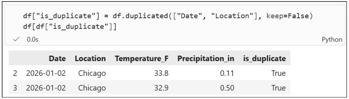
Since the original index is also visible in this output (duplicates are present in rows 2 and 3, for example), we could now manually make changes to these rows and delete them:
df.loc[2, "Temperature_F"] = 32.9
df = df.drop(index=3)
The combine_first method is also useful, as it combines two rows in a DataFrame into one. If we apply this method to a row from our DataFrame df.loc[2] and pass it a second row, the result is similar to the first row, but the values from the other row are used in places where NaN appears. For example, if we had one missing temperature value and one missing precipitation value, combine_first would combine these two rows into one, where the precipitation value from one row and the temperature value from the other row were used:
df.loc[2] = df.loc[2].combine_first(df.loc[3])
df = df.drop(index=3)
Here, too, we delete the row with index 3 after the combination process, since it’s the duplicate and is no longer needed.
You’ve now seen how to easily delete any of these rows when dealing with duplicates, how to merge them into a single row when dealing with missing values, and how to keep the rows with the largest or smallest value in a specific column by sorting and deduplicating. Of course, we can now come up with even more complex rules, such as combining where we have NaN values, taking the temperature value from the row where it’s highest, taking the lowest precipitation value, and, on Friday the 13th in leap years, always taking the precipitation value from the warmest location. There are, of course, no limits to your imagination here, but if you really need something like that, it’s best to ask a chat AI. Here is just a quick final example (more on the groupby method will follow later when we cover data analysis):
df = df.groupby(["Date", "Location"], as_index=False).agg({
"Temperature_F": "mean",
"Precipitation_in": "sum"
})
The rows in our DataFrame that share the same date and location are combined into a single row. The average is calculated from the individual temperature values, and the precipitation values are summed.
Identifying and Correcting Errors and Outliers
We’ve already looked at two types of errors in the data: missing values and duplicates. However, there are many other types of errors hiding in the data. Before we can begin troubleshooting and correcting errors, though, we first need to know what kinds of errors might even occur in our data. Unfortunately, there’s no magic command that will give us the erroneous rows if it isn’t clear in the first place what “erroneous” actually means. For an email address, it would be an error if an @ symbol is missing; temperature values should always fall within a certain range; and the date a person got married should always be later than their date of birth. Only after we’ve defined such error cases, we can specifically search for rows containing these errors and then look at how to fix them.
For the examples that follow, we’ll first create a DataFrame that contains a few errors:
df = pd.DataFrame({
'Date': ['2026-01-01', '2026-01-01', '2026-02-30'],
'Location': ['Chicago', 'Seattle ', 'chicago'],
'Temperature_F': [36.5, 35.2, 525.47],
'Precipitation_in': [0.0, 0.2, 0.1]
})
I have a DataFrame df with, among other things, a 'Location' column. Find the rows where the location is written in lowercase and correct the error by capitalizing the first letter, for example, “chicago” → “Chicago”.
You can do this quite easily in pandas. Here’s an example of how to find the rows where the location is in lowercase and correct them:
import pandas as pd
df = pd.DataFrame({
'Date': ['2026-01-01', '2026-01-01', '2026-02-30'],
'Location': ['Chicago', 'Seattle ', 'chicago'],
'Temperature_F': [36.5, 35.2, 525.47],
'Precipitation_in': [0.0, 0.2, 0.1]
})
# Find rows where the location is written in lowercase
mask = df['Location'].str[0].str.islower()
print("Rows with the location in lowercase:")
print(df[mask])
# Correct the lowercase locations (capitalize the first character)
df.loc[mask, 'Location'] = df.loc[mask, 'Location'].str.capitalize()
print("\nDataFrame after correction:")
print(df)
The filter predicate, which we always wrote directly in square brackets in previous examples, is stored here in a variable mask. We could also have written:
df[df['Location'].str[0].str.islower()]
This finds rows where the city is in lowercase. df['City'] is the entire city column. Str gives us access to string methods; in our case, [0] gives us the first character, and islower() allows us to check if it’s in lowercase. The capitalize method converts a string so that the first letter is now uppercase; "chicago" becomes "Chicago".
Did you actually notice that there’s a space after “Seattle” in our data (“Seattle ”)? Unfortunately, this is something that’s very often overlooked in practice. Especially when data is loaded from TSV, Excel, or similar files. You then wonder in later steps why a duplicate wasn’t detected and why there are still two rows with the location “Seattle” on the same day. After a long troubleshooting session, you eventually notice that one instance is the city "Seattle" and the other is "Seattle " with an invisible space. The best way to fix this is right at the start using the strip() method. strip() removes spaces at the beginning and end of a string:
df["Location"] = df["Location"].str.strip()
Now let’s address outliers in numerical columns. We want temperatures to always fall within a specific range and precipitation values to never be negative. If we do find such values, we’ll replace them with NaN so they don’t skew our calculations in later data analyses:
df.loc[(df["Temperature_F"] < -60) | (df["Temperature_F"] > 140),
"Temperature_F"] = np.nan
df.loc[df["Precipitation_in"] < 0, "Precipitation_in"] = np.nan
The value np.nan comes from the NumPy package. So, at the beginning of the Python program or at the top of the Jupyter Notebook, we must first import it using import numpy as np.
One final error that has crept into our sample dataset is the invalid date value "2026-02- 30". Dates and times shouldn’t be stored as strings in a DataFrame anyway; instead, it’s better to use the datetime data type. This also allows us to perform calculations on date values, for example, to add a week to a date or to check whether a date falls within a certain range. And incidentally, when converting strings containing a date, we can also see whether that date is invalid or not:
df["Date"] = pd.to_datetime(df["Date"], errors="coerce")
After this, the values in the date column no longer have the string data type, but rather the datetime data type. The option errors="coerce" ensures that invalid date values are converted to NaT (not a timestamp). Without this option, an error would be raised if there were invalid date values in the DataFrame, and the program would terminate.
Transforming Data into the Desired Format
So far, we’ve focused on removing errors from the data. From now on, we can say that we have error-free data. However, it’s still not in the format we’d like for performing adequate and convenient data analysis. For example, a temperature in degrees Celsius isn’t an error, but we’d much rather convert it to Fahrenheit:
df = pd.DataFrame({
'Date': ['2026-01-01', '2026-01-01', '2026-01-02'],
'Location': ['Chicago', 'Seattle', 'Chicago'],
'Temperature_C': [2.5, 1.8, 1],
'Precipitation_in': [0.0, 0.2, 0.11]
})
df["Temperature_F"] = df["Temperature_C"] * 9/5 + 32
After this transformation, our DataFrame contains both the old Temperature_C column with temperature values in degrees Celsius and the calculated Fahrenheit values in the Temperature_F column. We can keep the former column or remove it from the DataFrame using df = df.drop(columns=["Temperature_C"]).
Not only can calculations using +, -, *, and so on, be performed on entire columns, but mathematical functions can also be applied, for example, to round numbers. Using the round method, we can round the values in the column Precipitation_in to one decimal place:
df["Precipitation_in"] = df["Precipitation_in"].round(1)
This converts 0.11 to 0.1. Such data type–specific methods are available for numbers (e.g., round) and strings (e.g., strip(), which removes leading and trailing spaces), but also for columns containing dates or timestamps. The following command calculates the corresponding day of the week from the date and writes it to a new column:
df["Day of Week"] = pd.to_datetime(df["Date"]).dt.day_name()
More complex transformations can be performed by creating a function in which we define exactly how values should be converted. For example, you can assign countries to the categories "small", "medium", or "large" based on their population. For simpler cases, however, it’s sufficient to simply create a dictionary that specifies which values should be mapped to which new values:
state_map = {
"Chicago": "IL",
"Seattle": "WA",
"New York": "NY",
"Los Angeles": "CA",
"Houston": "TX"
}
df["State"] = df["Location"].map(state_map)
If a place name appeared in our data that isn’t present in the state_map, these rows would show a NaN in the State column.
The transformations shown are intended only as examples and are meant to serve as inspiration. Of course, many other transformations are possible, including significantly more complex ones. Chat-based AI tools are a great help here. It’s best to include the column names in the prompt—or even the entire output of df.info()—and describe exactly what should be transformed and how. Examples in the prompt are always helpful here as well, for example, “For Houston, the state should be TX.” Then the AI knows what typical values in the data look like and that states should be abbreviated.
(De)coding Categories
Decoding means that we have a kind of code or abbreviation in the data and want to convert it into what this abbreviation stands for. In the following DataFrame, the location 0 stands for Chicago and 1 for Seattle:
df = pd.DataFrame({
'Date': ['2026-01-01', '2026-01-01', '2026-01-02'],
'Location': [0, 1, 0],
'Temperature_F': [36.5, 35.2, 33.8],
'Precipitation_in': [0.0, 0.2, 0.11]
})
If we now want to have the full place names in the DataFrame, we can do this using the map method by passing it a dictionary. This dictionary specifies which abbreviation corresponds to which location:
location_map = {0: "Chicago", 1: "Seattle"}
df["Location"] = df["Location"].map(location_map)
The reverse process is called encoding. So, we have place names in the "Location" column but want to generate numbers instead—for example, 0 for Chicago and 1 for Seattle. In this case, we don’t need to pass a map; instead, we can have the codes generated automatically. The first value that appears in the DataFrame is then assigned the code 0. In our case, that would be Chicago, as before. All subsequent occurrences of Chicago are then assigned a 0 as well.
df["Location"] = df["Location"].astype("category").cat.codes
Now, of course, you might ask why you should do this at all. The goal of data cleaning and data transformations is, after all, to convert data into a format that allows you to work with it optimally, and there are some use cases where it’s easier to work with category numbers or numerical codes than with full-text values. This is particularly useful with machine learning algorithms. These algorithms often don’t care whether someone lives in Chicago or in Location 0. Many algorithms even require that the data be in numerical form. So, you have to perform such encoding beforehand, and when the algorithm later delivers a result, it may be necessary to decode it again. For example, if an AI algorithm predicts that a customer is highly likely to live in Location 0, you must convert this value back to the location name “Chicago” to make sense of the statement. Additionally, numbers save storage space compared to strings. This allows for more complex analyses to be performed with less storage requirements and thus potentially faster. Another use case is data anonymization. Once the data is encoded, it’s no longer possible to convert the numerical codes back to their original values.
Normalizing: Making Values Comparable
To avoid comparing apples to oranges, we must transform values so that they can be compared with one another at all, thereby enabling meaningful calculations. For example, if we merge two DataFrames from different sources and one uses temperatures in °C while the other uses °F, we must decide on a uniform format before merging them. We thus overcome the heterogeneity present in our data and make the data homogeneous.
Normalization is similar. We bring the data into a normal form—that is, a form that’s standardized in a certain way—so that it becomes comparable without changing the actual meaning of the values. A well-known example is min-max normalization. Behind this is an algorithm that identifies the smallest and largest values in a column, and then replaces every instance of that smallest value with a 0 and the largest value with a 1. All values in between are assigned a value between 0 and 1 accordingly. The formula behind it might look a bit strange, but ultimately it does exactly that:
df["Temp_minmax"] = (df["Temperature_F"] - df["Temperature_F"].min()) /
(df["Temperature_F"].max() - df["Temperature_F"].min())
If the lowest temperature in our dataset were 31 °F and the highest 105 °F, 31 °F would become 0, 68 °F would become 0.5 (because (68 – 31) / (105 – 31) = 0.5), and 105 °F would become 1.
Such normalizations are also frequently performed when AI algorithms are used. Many machine learning algorithms require that the data be normalized beforehand. Furthermore, values between 0 and 1 are often easier to understand. For example, is 103 °F a lot? That depends on the context. Is 0.98 a lot (on a scale from 0 to 1)? Yes, definitely! Outliers— both below and above the mean—are easier to spot in normalized values, and when creating charts and visualizations, normalized values provide a useful and consistent scale right out of the box.
In addition to min-max normalization, there are other normalization methods, such as the Z-score, the L2 norm, log normalization, calculating the proportion of the total sum, and many more. Each has its pros and cons. With log normalization, for example, outliers stand out more. But I don’t need to go into detail here—if you want to do something like this, you probably already know what you’re doing.
Editor’s note: This post has been adapted from a section of the book Python for AI and Data Analysis: The Practical Guide for Business and Science by Johannes Schildgen. Prof. Dr. Schildgen is a professor of databases, specializing in big data, at Ostbayerische Technische Hochschule (OTH) Regensburg (the Regensburg University of Applied Sciences). For nearly a decade, he has taught Python programming to students. As a keynote speaker, he regularly delivers engaging talks on digitalization, artificial intelligence, and other IT-driven future trends.




Comments